Wednesday, July 8, 2015

Contribution of LFP dynamics to single-neuron spiking variability in motor cortex during movement execution

My first Ph.D. publication is out! Contribution of LFP dynamics to single-neuron spiking variability in motor cortex during movement execution explores how the activity of individual neurons in motor cortex is related to population activity, as measured by electrical Local Field Potentials (LFPs). 

[get PDF] 

How do the actions of individual cells combine to create the emergent dynamics that underlie perception, thought, and action? To answer this question, we should study populations of single neurons, and ask how their activity is related to measures of collective population dynamics. This study was a collaboration between the Truccolo and Donoghue labs, and looked at neural population recordings from primate motor cortex during movement.

We found that the activity of single cells was tightly coupled to population activity as measured by LFPs, and that both of these signals were closely realated to movement. This suggest that, during movement execution, collective dynamics reflected in motor cortex LFPs mostly reflect the sensorimotor processes directly controlling movement output. It also suggests that primary motor cortex isn't engaged in other activities like cognition or future planning, while executing movements.

Importantly, we considered both past and future movement in this analysis, and found that single neurons and LFPs both contain information about recent and upcoming movements. This is consistent with the view that motor cortex acts as a dynamical pattern generator.

Many thanks to Carlos Vargas-Irwin, John P. Donoghue, and Wilson Truccolo. The article is open access, and you can also grab the PDF from Github. The paper can be cited as:

Rule, M.E., Vargas-Irwin, C., Donoghue, J.P. and Truccolo, W., 2015. Contribution of LFP dynamics to single-neuron spiking variability in motor cortex during movement execution. Frontiers in systems neuroscience, 9, p.89. 


Figure 4. Breakdown of LFP predictive power by frequency band and LFP feature. Box-plots over the population of isolated units (all sessions combined) showing the predictive power of models based on phase, amplitude, or analytic signal features in isolation from each of eight LFP bands. To better assess the individual predictive power of each LFP feature, models were fitted for each feature separately. Certain features, such as the instantaneous phase and analytic signal for the 0.3–2 Hz band, as well as the analytic signal amplitude modulation above 100 Hz, consistently predict spiking across all animals and areas.

Wednesday, April 1, 2015

Directional statistics for spatiotemporal wave analysis

I've been searching for a good distribution that can be used to summarize how the distribution of phases and amplitudes evolves during transient synchronization events of beta (~20 Hz) local field potentials (LFP) in motor cortex. So far, it seems difficult to find a single distribution family that works in all cases. 

Spatiotemporal wave activity in beta oscillations in motor cortex can be described in terms of the beta-band analytic LFP signal, which has both a magnitude and a phase, and who's real part is equal to the time-domain value of the beta-filtered signal. 

\begin{equation}z_k(t) = \beta_k (t) + i\cdot  \operatorname{Hilbert}(\beta_k)(t) = r_k(t) e^{i \theta_k(t)},\\\textrm{ where $k$ indexes over channels}\end{equation}

Circular statistics can be used to summarize the distribution of analytic signal phase, in order to detect synchrony and wave events.

[read more in the PDF


Figure 2: Neither the complex Gaussian nor log-polar statistics perfectly describe the distributions of analytic signal. In these plots, the black ellipse represents a complex Gaussian model of the data, with the ellipse boundary at one standard deviation, and the ellipse axes representing the eigenvectors of the covariance matrix $\Sigma$. The cyan contours represent a log-polar model of the data, which uses the mean and standard deviation of the log-amplitude, as well as the circular mean and standard deviation of the phases, to model the data in log-polar space. (a) When phase is concentrated, and not correlated with amplitude, both the log-polar statistics and the complex Gaussian distribution describe the data well. (b) When phase and amplitude are correlated, the log-polar model cannot capture the phase-amplitude dependence. (c) During traveling wave events, signal amplitude is high, and there is dispersion in phase. In these cases, the log-polar statistics are more appropriate than the complex Gaussian. (d) Traveling wave events appear to often evolve from states that show a mixture of synchrony and standing wave dynamics. The log-polar statistics break down when the phase distribution is bimodal, but the complex Gaussian can describe these states well. (e) At low signal amplitudes, the system is often asynchronous, and the phase and amplitude of the log-polar model are poorly defined. (f) Although rare or absent in our data, a hypothetical distribution with uniform phase and concentrated amplitude could occur, say, during traveling wave events with short wavelength. In this case, the complex Gaussian model is especially bad.

Friday, March 20, 2015

Three unbiased estimators of spike-field coherence

[get notes as PDF]

In these notes we show a simplified expression for the Pairwise Phase Consistency (PPC) measure of Vinck et al. (2010). We illustrate it's relation to a bias-corrected spike-field coherence measure from Grasse et al. (2010), and discuss an third notion of spike-field coherence that is intermediate between the two. 

Here, we use the term "event-triggered" rather than "spike-triggered", because we want to apply these measures to neural events other than spikes (e.g. beta-frequency transients in motor cortex).

Pairwise Phase Consistency

Vinck et al. (2010) define Pairwise Phase Consistency (PPC) as the expected dot product between all pairs of (spike-triggered) phase measurements. 

\[\hat\Upsilon = \frac 2 {N(N-1)} \sum_{j=1..N-1} \sum_{k=j+1..N} \cos(\theta_j - \theta_k)\]

There is an alternative way to express PPC that is faster to calculate, and also reveals a relationship between PPC and similar alternatives. 

Motor cortex LFP spatiotemporal dynamics in a cued grasp with instructed delay task

Update: Portions of these notes have now been published in the Journal of Neurophysiology as  "Dissociation between sustained single-neuron spiking and transient β-LFP oscillations in primate motor cortex" and "Phase reorganization leads to transient β-LFP spatial wave patterns in motor cortex during steady-state movement preparation".

[get notes as PDF]

Task-locked modulations in neural activity

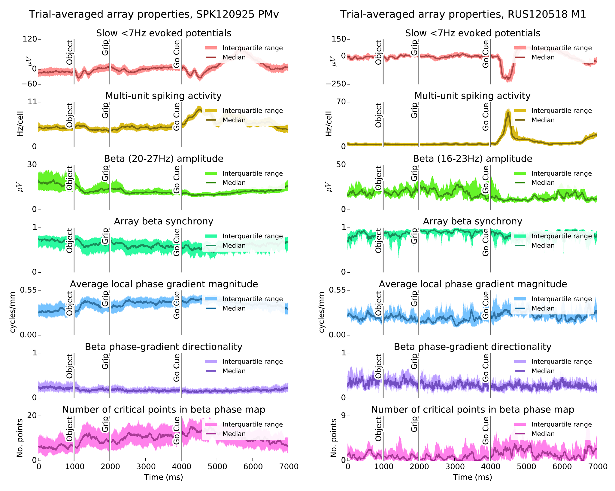
The Cued Grasp with Instructed Delay (CGID) task reliably elicits task-locked activity in all three motor areas (M1, PMd, PMv).

  • Consistent with prior literature, the movement period of the CGID task is marked by slow motor evoked potentials (Fig. 2), increased single-unit firing rates (Fig. 3), and beta suppression (Fig. 4).
  • Beta oscillations are enhanced during the first four seconds of the task, although there are some differences between subjects.
  • The average level of beta-LFP synchrony is correlated with beta-LFP power, and varies across phases of the task.
  • We find no evidence of task-locked phase resetting of beta LFP oscillations
  • The spatiotemporal structure of beta-LFP waves is correlated with amplitude and synchrony, with lower amplitudes reflecting more complex wave structures, and higher amplitudes as more synchronous.

figure1

Figure 1: The CGID task reliably elicits evoked potentials, which correlate with beta suppression. In subject S, beta power is strongest in the first second before object presentation. In subject R, beta oscillations are more variable, with somewhat stronger power between the grip and go cues. In both animals, high beta power appears to correspond to periods of higher beta synchrony, and larger phase gradient directionality, a measure of how much LFP activity resembles a plane wave. Conversely, increases in the average magnitude of the Hilbert phase gradient, which summarizes how quickly beta phase changes over the array, and in the number of critical points in the Hilbert phase gradient, which summarizes the complexity of the beta spatiotemporal wave patterns, correspond to periods of beta suppression.

Tuesday, September 9, 2014

A mechanism for persistent memory in oscillatory networks

I just finished the Methods in Computational Neuroscience "bootcamp". It was intense, but valuable—I can recommend that any student/postdoc who wants to get started in the field take it. 

For a course project, I extended previous work, which showed that oscillatory drive can excite patterned instabilities in visual cortex. These patterns constitute attractor states that are stabilized by an external oscillatory drive. The project explored the idea that similar oscillation-stabilized attractors might serve as a flexible working memory. 

(Unfortunately, these notes are rather brief and incomplete as I never had the time to write this up properly. )

Selective, short-term maintenance of attractor states is important for working memory in neural systems. Neural networks, however, are typically stabilized by feedback inhibition. The delays in this inhibition lead to unavoidable oscillations. 

This project demonstrate a scenario where the attractor dynamics associated with a working memory are not fixed points, but instead fixed limit cycles embedded within a population oscillation. 

External oscillatory drive, perhaps e.g. an attention signal, can switch such a network from a "read-in" mode, in which the system responds to external input, and a "hold" model, in which the system retains a memory of its past states. These concepts may underlie flexible working memory solutions that can coexist with population oscillations.

To better understand the mechanisms underlying this, we explored a switched piece-wise linear model that captured the qualitative dynamics of the original system. We found that firing-rate nonlinearities with positive curvature are important for allowing a synchronous (non-selective) external signal to excite the asymmetric network states associated with a memory trace. 

[get writeup PDF]

[get presentation slides]

Preview: Figure 4

Figure 4: Many-population generalization of the two-population model of Rule et al. (2011), serving as a working memory. Starting from rest, a stimulus is delivered to the first oscillator (green) for $t\in[300,500)$ ms. We test the stability of this stimulus-driven network response during a hold period $t\in[500,1500)$ ms. Without oscillatory drive (top), the memory fades in a few cycles. Periodic stimulation (bottom) preserves the memory. Rightmost plots show the phase-plane dynamics during the readout period $t\in[1000,1500)$. The top system, without drive, has returned to rest. The driven system shows a stable limit cycle, with higher firing rates in the population that initially received the stimulus.

Saturday, June 29, 2013

Invent-abling: enabling inventiveness through craft

This latest paper, "Invent-abling: enabling inventiveness through craft", is a departure from the usual science.  

For the outreach component of the NHS Graduate Research Fellowship Program, and I've teamed up with Deren Güler to explore ways to make early STEM education more engaging and accessible for a diverse array of young people. 

We've been running workshops that merge electronics educational lessons with crafting—origami, sewing, etc. The idea was that STEM education disguised as arts-and-crafts would engage children of all genders and diverse backgrounds more equally. We felt that this would be a more natural and accessible, in contrast to simply, say, making pink breadboards. 

We learned a lot, especially about circumventing biases and preconceptions concerning gender identity and patterns of play. The hands-on and open-ended approach of these workshops was also inclusive of children with differing skill levels. We presented what we've learned at the 12th International Conference on Interaction Design and Children, as a conference paper [PDF]. You can cite it as: 

Guler, S.D. and Rule, M.E., 2013, June. Invent-abling: enabling inventiveness through craft. In Proceedings of the 12th International Conference on Interaction Design and Children (pp. 368-371). 

The plan for the future is to establish a LLC to produce the lesson materials and components, and provide these materials to educators who wish to host similar workshops.

Edit, circa 2019: Epilogue

Thanks to Deren's dedication and persistence, this outreach program has grown into a full-fledged company, Teknikio. Teknikio provides both individual kits and classroom kits for educators. In the years since the first workshops, we've developed new workshops added many more re-usable components for kids to incorporate into their inventions.

The Gordon and Betty Moore Foundation SPARK Award was instrumental in providing start-up capital. In 2018, Teknikio received an NSF Small Business Innovation Research (SBIR) phase I grant to prototype an Internet-of-Things (IoT) kit for the classroom. In 2019, this grant was extended to a phase II award to begin commercialization. Great things start small.


Monday, April 22, 2013

Calculating the AUC for Poisson GLM models of deconvolved spike-train data

These notes provide a function for calculating the AUC for a Poisson regression that works when the spike counts are given only up to some (unknown) normalization constant. Skip to the end for the Python code.

Poisson regression and point processes

Neuroscientists use Poisson regression (in the continuous limit: Poisson point process ) to assess the correlation between neuronal spiking and other experimental covariates. These models are well suited to the scenario in which spikes are binary all-or-nothing events, recorded based on electrical potentials.

The area under the receiver operating characteristic curve

It is common to assess the performance of a Poisson GLM using the Area Under the receiver-operator-characteristic Curve (AUC) .

Definition of the AUC: The AUC is defined as the probability that a randomly-sampled (true-negative, true-positive) pair will be correctly ranked by the predicted firing-rates. We can calculate it by integrating over all such pairs. We will work in continuous time $t\in[0,T]$ for an experiment with duration $T$.

Denote the sets of true positives and true negatives as $t_p\in\mathcal T_p$ and $t_n\in\mathcal T_n$, respectively. Consider a generic model $\lambda(t)$ which predicts the spiking probability at time $t$. Generically, the AUC can be calculated by integrating over all pairs $(t_p,t_n)$ of positive and negative examples:

\begin{equation} \begin{aligned} \text{AUC}(\lambda,\mathcal T_p,\mathcal T_n) &= \Pr\big\{ \lambda(t_n) < \lambda(t_p) \text{ for }t_n\in\mathcal T_n \text{ and }t_p\in\mathcal T_p \big\} \\ &= \frac{1}{|\mathcal T_n|} \frac{1}{|\mathcal T_p|} \int_{t_n\in\mathcal T_n} \int_{t_p\in\mathcal T_p} \delta_{\lambda(t_n)<\lambda(t_p)}, \end{aligned} \label{auc0} \end{equation}

[auc0]

where $\delta_{u{>}v}$ as an indicator function, which is $1$ if $u{>}v$.

Why use the AUC?

Because it depends only on the relative ranks of predicted firing rates, AUC is insensitive to errors in predicting a cell's mean rate, firing-rate variance, or any other strictly increasing transformation of the true rates. These properties make the AUC a desirable performance metric if we only care how well a GLM predicts neuronal tuning in a very general sense. It can be viewed as a type of nonlinear (rank) correlation between the test data and model predictions.

Calcium imaging yields fractional spike counts

Calcium fluorescence imaging has emerged as a standard method for simultaneously recording from large populations of neurons. Since calcium concentrations change relatively slowly following spiking, spike times are recovered indirectly by deconvolving calcium fluorescence signals.

These time-series of deconvolved spikes are sparse, with most entries zero. However, when spikes are detected, they are often detected with a fractional (non integer) value. This introduces some subtleties when working with point-process models, which are defined in terms of all-or-nothing (integer) events.

In practice, non-integer spike counts are no issue for the Poisson regression. Although a rigorous definition of the Poisson distribution is defined only on integers, it can be evaluated for any non-negative real number. This is technically improper, but works just as well and is commonly used in quasi-Poisson regression .

However, integrating commonly used measurements of model performance with fractional spike counts is slightly more subtle.

The AUC for continuous-time spiking data

For spiking data, the "true positives" are the spike times, and the "true negatives" are times when a neuron does not spike. We will work in continuous time, in which a spike train can be treated as a sum of delta distributions at each spike time, $y(t) = \sum_{t_s\in\text{spike times}} \delta(t-t_s)$.

In this continuous case, the duration of spikes is infinitesimal. This means that the set of true positives (i.e. times containing a spike) is of measure zero, compared to the measure of the time-duration of the experiment. In other words, the probability that a given time-point $t_n$ corresponds to a true negative, $\operatorname P_{t_n\in\mathcal T_n}$ is effectively $1$. True negatives are therefore uniformly distributed, with $\operatorname P_{t_n=t | t_n\in\mathcal T_n}= 1/T$.

In contrast, the true positives are a discrete set of $K = |\mathcal T_p|$ spikes, turning the second integral in $\eqref{auc0}$ into a sum. For a continuous spiking time-series, the AUC in $\eqref{auc0}$ can then be written in terms of the spike times $t_k\in\mathcal T_p$, $k\in\{1,\dots,K\}$ as:

\begin{equation} \begin{aligned} \text{AUC}(f,\mathcal T_p) &= \frac{1}{TK} \int_{t_n\in[0,T]} \sum_{k=1}^K \delta_{\lambda(t_n)<\lambda(t_k)} \\ &= \frac{1}{TK} \sum_{k=1}^K \int_{0}^{T} \delta_{\lambda(t)<\lambda(t_k)} \,dt. \end{aligned} \label{auc0b} \end{equation}

[auc0b]

The AUC for deconvolved spikes

Deconvolved spikes from fluorescence data do not recover the true spikes counts $y(t)$, only a non-negative time-series $y(t)$ that is proportional to them (and is not quantized).

This is no problem in practice. To compute the AUC, we only need the density of true positive events per unit time, not their absolute number. The density of true positives per unit time is simply $y$ divided by its sum:

\begin{equation} \begin{aligned} \Pr(\,t_p{=}t \,|\, t_p{\in}\mathcal T_p\,) = \frac {y(t)} {\int_{dt} y(t)} \end{aligned} \label{pt} \end{equation}

[pt]

To calculate the AUC, we could sample $t_n\in\mathcal T_n$ uniformly over $[0,T]$, and sample $t_p\in\mathcal T_p$ using the normalized deconvolved spike counts, $p_t$. We can compute the expectation of this sampling exactly by integrating over the joint distributions of true positives and negatives.

\begin{equation} \begin{aligned} \text{AUC}(\lambda,y) &= \frac 1 {T \int_{dt} y(t)} \int_0^T y(t_p) \int_0^T \delta_{\lambda(t_p){>}\lambda(t_n)} \,dt_n\,dt_p, \end{aligned} \label{auc1} \end{equation}

[auc1]

We'd like to transform this equation into a nicer form, getting rid of that $\delta$ and producing something we can type into the computer.

Define $\operatorname s(t) \in [0,1]$ as the relative rank-ordering of $\lambda(t)$, which starts at 0 for the smallest $\lambda(t)$, and counts up to $1$ for the largest $\lambda(t)$:

\begin{equation} \begin{aligned} \operatorname s(t) &:= \frac {\text{rank of $\lambda(t)$}} {T} = \frac 1 T \int_0^T \delta_{\lambda(t){>}\lambda(\tau)}\,d\tau \end{aligned} \label{s} \end{equation}

[s]

Using $\operatorname s(t)$, we can write the AUC as defined in $\eqref{auc1}$ as:

\begin{equation} \begin{aligned} \text{AUC}(\lambda,y) &= \int_0^T p(t) s(t)\,dt \end{aligned} \label{auc2} \end{equation}

[auc2]

In discrete time, $\eqref{auc2}$ reduces to an average of the ranks $s_t\in[0,1]$, weighted by the deconvolved spike counts $y$. Here it is in Python:

def auc(λ,y):
    '''
    Area Under the ROC Curve (AUC) for deconvolved spike data. 

    Parameters
    ----------
    λ: 1D np.float32, length NSAMPLES
        Predicted scores for each datapoint
    y: 1D np.float32, length NSAMPLES
        Estimated spike counts for each datapoint

    Returns
    -------    
    AUC: float
        Area under the receiver-operator-characteristic curve. 
    '''
    # Cast to numpy arrays
    λ   = np.array(λ).ravel()
    y   = np.array(y).ravel()

    # Ignore NaNs
    bad = ~np.isfinite(λ)|~np.isfinite(y)
    λ   = λ[~bad]
    y   = y[~bad]

    # AUC is undefined if there are no positive examples
    d   = np.sum(y)
    if d<=0: return NaN

    # Density of true positives per timepoint
    py  = y/d

    # Convert scores to fractional ranks
    rs  = scipy.stats.rankdata(λ)/len(λ)

    AUC = np.average(rs,weights=py)
    return AUC