These notes explore a deterministic limit of Autoregressive Point-Process Generalized Linear Model (AR-PPGLM) of a spiking neuron. We consider a Poisson point process that is either strongly driven or strongly suppressed, and take a limit where spiking output becomes deterministic (and instantaneous rates diverge). This deterministic limit is of interest in clarifying how AR-PPGLM models relate to deterministic models of spiking.
Showing posts with label notes. Show all posts
Showing posts with label notes. Show all posts
Thursday, June 20, 2019


Tuesday, February 5, 2019
Moment equations for an autoregressive point process with an absolute refractory period
These notes extend the autoregressive point-process moment closures derived in Rule and Sanguinetti (2018) to models that include an absolute refractory period via a gating term that sets the rate to zero after a spike.
Tuesday, January 8, 2019
Gaussian moment-closures for autoregressive GLM population models
In Rule and Sanguinetti (2008) "Autoregressive Point Processes as Latent State-Space Models" (more at the blog post) we developed moment-closure approximations for the time-evolution of the moments of Autoregressive Point-Process Generalized Linear Models (AR-PPGLMs) of neural activity. These notes generalize these approximations for AR-PPGLM models of neural ensembles . For networks of linear-nonlinear "neurons", the derivations are very similar to the single-neuron case presented in the paper.
Tuesday, July 10, 2018
Approximations of the measurement update and model likelihood for nonlinear spatiotemporal Cox processes
Epilogue: These notes were part of a project to infer unobserved ("latent") states in a neural field model, as well as the parameters of that model, from spiking observations. It has since been published. Ultimately, for speed we ended up selecting the Laplace approximation for the measurement update, solved via Newton-Raphson.
We are interested in approximations to the measurement update for a spatially-extended latent-variable point-process, where the latent variables are also spatial fields that undergo dynamics similar to chemical reaction-diffusion systems.
The latent variables or fields are concentrations, activations, or some similar physical quantity. They are therefore constrained to be non-negative, and also typically must obey conservation laws. Additionally, the observed point-process intensity field must also be constrained to be non-negative.
Such systems arise in chemical reaction diffusion systems, epidemiological models, and neural field models, where the measurement is a point-process that is coupled indirectly to the latent spatiotemporal system.
Saturday, February 4, 2017
System-size expansion and Gaussian moment closure for Quiescent-Active-Refractory model
Epilogue: These notes concern the system size expansion and moment closure later published as "Neural field models for latent state inference: Application to large-scale neuronal recordings" [pdf] (more)
These notes derive the Kramers-Moyal system size expansion and approximate equation for the evolution of means and covariances of a single-compartment neural mass model with Quiescent (Q), Active (A), and Refractory (R) states. The derivations here are identical to the standard ones for the Susceptible (S), Infected (I), and Recovered (R) (SIR) model commonly used in epidemiology.
Friday, March 20, 2015
Motor cortex LFP spatiotemporal dynamics in a cued grasp with instructed delay task
Update: Portions of these notes have now been published in the Journal of Neurophysiology as "Dissociation between sustained single-neuron spiking and transient β-LFP oscillations in primate motor cortex" and "Phase reorganization leads to transient β-LFP spatial wave patterns in motor cortex during steady-state movement preparation".
Task-locked modulations in neural activity
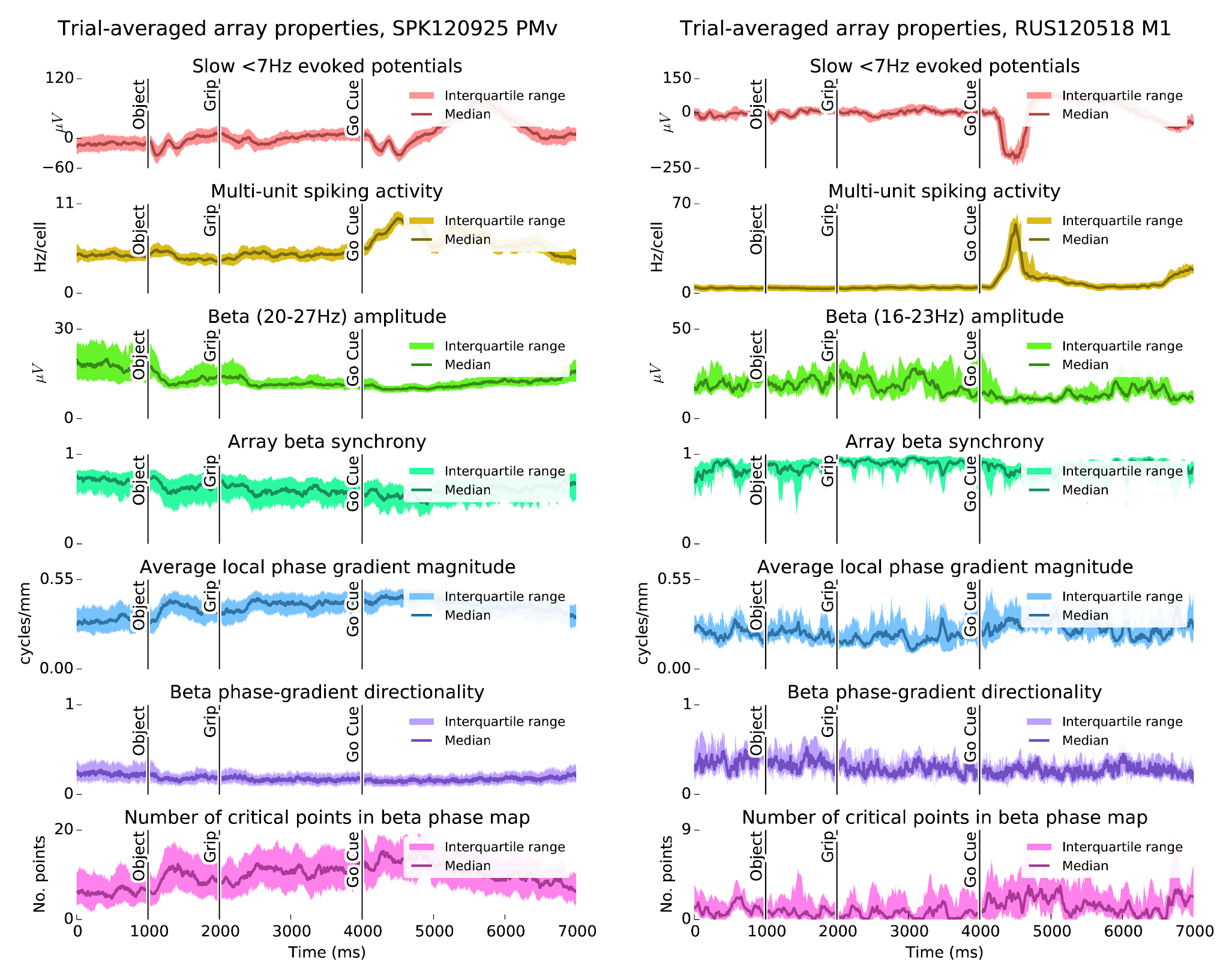
The Cued Grasp with Instructed Delay (CGID) task reliably elicits task-locked activity in all three motor areas (M1, PMd, PMv).
- Consistent with prior literature, the movement period of the CGID task is marked by slow motor evoked potentials (Fig. 2), increased single-unit firing rates (Fig. 3), and beta suppression (Fig. 4).
- Beta oscillations are enhanced during the first four seconds of the task, although there are some differences between subjects.
- The average level of beta-LFP synchrony is correlated with beta-LFP power, and varies across phases of the task.
- We find no evidence of task-locked phase resetting of beta LFP oscillations
- The spatiotemporal structure of beta-LFP waves is correlated with amplitude and synchrony, with lower amplitudes reflecting more complex wave structures, and higher amplitudes as more synchronous.
Figure 1: The CGID task reliably elicits evoked potentials, which correlate with beta suppression. In subject S, beta power is strongest in the first second before object presentation. In subject R, beta oscillations are more variable, with somewhat stronger power between the grip and go cues. In both animals, high beta power appears to correspond to periods of higher beta synchrony, and larger phase gradient directionality, a measure of how much LFP activity resembles a plane wave. Conversely, increases in the average magnitude of the Hilbert phase gradient, which summarizes how quickly beta phase changes over the array, and in the number of critical points in the Hilbert phase gradient, which summarizes the complexity of the beta spatiotemporal wave patterns, correspond to periods of beta suppression.
Tuesday, September 9, 2014
A mechanism for persistent memory in oscillatory networks
I just finished the Methods in Computational Neuroscience "bootcamp". It was intense, but valuable—I can recommend that any student/postdoc who wants to get started in the field take it.
For a course project, I extended previous work, which showed that oscillatory drive can excite patterned instabilities in visual cortex. These patterns constitute attractor states that are stabilized by an external oscillatory drive. The project explored the idea that similar oscillation-stabilized attractors might serve as a flexible working memory.
(Unfortunately, these notes are rather brief and incomplete as I never had the time to write this up properly. )
Selective, short-term maintenance of attractor states is important for working memory in neural systems. Neural networks, however, are typically stabilized by feedback inhibition. The delays in this inhibition lead to unavoidable oscillations.
This project demonstrate a scenario where the attractor dynamics associated with a working memory are not fixed points, but instead fixed limit cycles embedded within a population oscillation.
External oscillatory drive, perhaps e.g. an attention signal, can switch such a network from a "read-in" mode, in which the system responds to external input, and a "hold" model, in which the system retains a memory of its past states. These concepts may underlie flexible working memory solutions that can coexist with population oscillations.
To better understand the mechanisms underlying this, we explored a switched piece-wise linear model that captured the qualitative dynamics of the original system. We found that firing-rate nonlinearities with positive curvature are important for allowing a synchronous (non-selective) external signal to excite the asymmetric network states associated with a memory trace.
Preview: Figure 4
 |
| Figure 4: Many-population generalization of the two-population model of Rule et al. (2011), serving as a working memory. Starting from rest, a stimulus is delivered to the first oscillator (green) for $t\in[300,500)$ ms. We test the stability of this stimulus-driven network response during a hold period $t\in[500,1500)$ ms. Without oscillatory drive (top), the memory fades in a few cycles. Periodic stimulation (bottom) preserves the memory. Rightmost plots show the phase-plane dynamics during the readout period $t\in[1000,1500)$. The top system, without drive, has returned to rest. The driven system shows a stable limit cycle, with higher firing rates in the population that initially received the stimulus. |
Wednesday, January 16, 2013
Impact of redundancy on stable decoding
Neural activity is redundant: many states in motor cortex can generate similar movements. When we record from motor cortex, we capture only a small fraction of the total neurons. Redundancy makes it possible to observe the overall state of motor cortex from limited observations, but might also impair the generalization performance of a linear decoder.
Consider two neurons, $A$ and $B$, that combine linearly to produce movement $C{=}\alpha_1 A{+} \alpha_2 B$. (Perhaps both neurons drive the same targets in spinal cord.) An animal could use any linear combination of activations of units $A$ and $B$ to perform behavior $C$, so long as the sum $\alpha_1{+}\alpha_2$ is constant. What if there is an unobserved variable $\gamma$ that sets whether neuron $A$ or $B$ is used more (Fig. 1)?
 |
| Figure 1: (simulated hypothetical scenario) Neural signals $A$ and $B$ combine linearly according to weight $\gamma$ to form behavioral output $C=\gamma A + (1-\gamma) B$. Parameter $\gamma$ modulates sinusoidally between $0.25$ and $0.75$. |
Wednesday, October 31, 2012
Sometimes the spike-triggered average is just as good as Poisson GLMs for spike-train analysis
(hopefully no major mistakes in this one; get PDF here)
The Poisson GLM for spiking data
Generalized Linear Models (GLMs) are similar to linear regression, but account for nonlinearities and non-uniform noise in the observations. In neuroscience, it is common to predict a sequence of spikes $Y=\{y_1,..,y_T\}$, $y_i\in\{0,1\}$, from a series of observations $X=\{\mathbf x_1,..,\mathbf x_T\}$, using a Poisson GLM:
$$ \begin{aligned} y_i &\sim \operatorname{Poisson}(\lambda_i\cdot\Delta t) \\ \lambda_i &= \exp\left( \mathbf a^\top \mathbf x_i + b \right) \end{aligned} $$These models are fit by minimizing the negative log-likelihood of the observations, given the vector of regression weights $\mathbf a$ and mean offset parameter $b$:
Saturday, January 14, 2012
Bayesian approach to point-process generalized linear models
I've been learning about generalized linear models and Bayesian approaches for doing statistics on spike train data, in the Truccolo lab. Here are some notes on the subject.
In neuroscience, we are interested in the problem of how neurons encode, process, and communicate information. Neurons communicate over long distances using brief all-or-nothing events called spikes. We are often interested in how the spiking rate of a neuron depends on other variables, such as stimuli, motor output, or other ongoing signals in the brain.
To model this, we consider spikes as events that occur at a point in time with an underlying variable rate, or conditional intensity, $\lambda$. There are many approaches to estimating $\lambda$. These notes cover point-process generalized linear models, and Bayesian approaches. These are closely related, and in some cases the same thing.
Tuesday, November 8, 2011
Point-Process Generalized Linear Models (PPGLMs) for spike train analysis
Get these notes as PDF here.
In neuroscience, we often want to understand how neuronal spiking relates to other variables. For this, tools like linear regression and correlation often work well enough. However, linear approaches presume that the underlying relationships are linear and the noise is Gaussian, neither of which are true for neural datasets. The Generalized Linear Model (GLM) extends linear methods to better account for nonlinearity and non-Gaussian noise.
GLMs for spike train analysis
We're interested in understanding how a neural spike train $y(t)$ relates to some other covariates $\mathbf x(t)$. In continuous time, a spike train is modeled as a train of impulses at each spike time $t_i$, $y(t)=\sum_i \delta(t-t_i)$. In practice, we always work in discrete time. It is common to choose a time step $\Delta t$ small enough so that at most one spike occurs in each time bin.
Two types of GLM that are common in spike train analysis:
- The Poisson GLM assumes that spikes arise from an inhomogeneous Poisson process with time-varying rate $\lambda(t)$ that depends log-linearly on the covariates $\mathbf x(t)$. In practice, it is common to treat the Poisson GLM in discrete time by assuming that the rate $\lambda(t)$ is constant within each time-bin:
- The Bernoulli GLM models each time-bin of a binary, discrete-time spike train $y_t\in\{0,1\}$ as a Bernoulli "coin flip" with $\Pr(y{=}1)=p$.
Maximum likelihood
GLMs are typically estimated using maximum likelihood when testing how covariates $\mathbf x(t)$ influence spiking. (Other fitting procedures may be more appropriate when GLMs are used to model spiking dynamical systems.) The maximum likelihood procedure finds the weights $\mathbf w$ that maximize the likelihood of observing spike train $\mathbf y=\{y_1,..,y_T\}$, given covariates $\mathbf X = \{ \mathbf x_1,..,\mathbf x_T\}$, over all $T$ recorded time-bins.
\begin{equation*} \begin{aligned} \mathbf w = \underset{\mathbf w}{\operatorname{argmax}} \Pr( \mathbf y | \mathbf w, \mathbf X) \end{aligned} \end{equation*}In practice, likelihood maximization is typically phrased in terms of minimizing the negative log-likelihood. Working with log-likelihood is more numerically stable, and the problem is phrased as minimization so that it is more straightforward to plug-in to off-the-shelf minimization code.
\begin{equation*} \begin{aligned} \mathbf w = \underset{\mathbf w}{\operatorname{argmin}} -\ln\Pr( \mathbf y | \mathbf w, \mathbf X) \end{aligned} \end{equation*}Assuming observations are independent, the negative log-likelihood factors into a sum over time-points. Equivalently, one can minimize the average negative log-likelihood, over samples, $- \left< \ln\Pr( y_t | \mathbf w, \mathbf x_t) \right>$. The maximum likelihood parameters are typically solved for via gradient descent or the Newton-Raphson method . This requires computing the gradient and hessian of the negative log-likelihood.
Gradient and Hessian for the Poisson GLM
We can calculate the gradient and Hessian for the Poisson GLM by substituting the Poisson probability density function, $\Pr(y)=\lambda^y e^{-\lambda}/y!$, in to our expression for the negative log-likelihood:
\begin{equation*} \begin{aligned} -\left<\ln\Pr( y_t | \mathbf w, \mathbf x_t)\right> &= \left<\lambda_t - y_t \ln(\lambda_t) - \ln(y!)\right> \end{aligned} \end{equation*}Because the term $\ln(y!)$ does not depend on $\mathbf w$, we can ignore it without affecting the location of our optimum. Substituting in $\lambda = \exp(\mathbf w^\top \mathbf x)$, we get:
\begin{equation*} \begin{aligned} \ell &= \left< \exp(\mathbf w^\top \mathbf x) - y_t \mathbf w^\top \mathbf x_t\right> \end{aligned} \end{equation*}Finding weight $\mathbf w$ that minimize $\ell$ is equivalent to solving for the maximum-likelihood weights. The gradient and Hessian of of $\ell$ in $\mathbf w$ are:
\begin{equation*} \begin{aligned} \frac {\partial \ell} {\partial w_i} &= \left<[ \exp(\mathbf w^\top \mathbf x_t) - y_t] x_i \right> = \left<(\lambda_t - y_t) x_i \right> \\ \frac {\partial \ell} {\partial w_i \partial w_j} &= \left<[ \exp(\mathbf w^\top \mathbf x_t) ] x_i x_j \right> = \left< \lambda_t x_i x_j \right> \end{aligned} \end{equation*}In matrix notation, these derivatives can then be written as:
\begin{equation*} \begin{aligned} \nabla \ell &= \langle \mathbf x( \lambda - y) \rangle \\ \mathbf H \ell &= \langle \lambda \mathbf x \mathbf x^\top \rangle \end{aligned} \end{equation*}Gradient and Hessian for the Bernoulli GLM
The Bernoulli GLM is similar, with the observation probability given by the Bernoulli distribution $\Pr(y) = p^y (1-p)^{1-y}$
\begin{equation*} \begin{aligned} \left< -\ln\Pr( y_t | \mathbf w, \mathbf x_t) \right> &=- \left< y_t \ln(p_t) + (1-y_t) \ln(1-p_t) \right> \\&=- \left< y_t \ln\left(\tfrac{p_t}{1-p_t}\right) + \ln(1-p_t) \right> \end{aligned} \end{equation*}Then, using $p = [1 + \exp(-\mathbf w^\top \mathbf x)]^{-1}$, i.e. $\mathbf w^\top \mathbf x = \ln[p/(1-p)]$, we get:
\begin{equation*} \begin{aligned} \ell &= \left< \ln[1+\exp(\mathbf w^\top \mathbf x_t)] - y_t \mathbf w^\top \mathbf x_t \right> \end{aligned} \end{equation*}The gradient and Hessian of of $\ell$ in $\mathbf w$ are:
\begin{equation*} \begin{aligned} \frac {\partial \ell} {\partial w_i} &= \left< \left[\frac{\exp(\mathbf w^\top \mathbf x_t)}{1+\exp(\mathbf w^\top \mathbf x_t)} - y_t\right] x_i\right> \\&= \left<(p_t - y_t) x_i\right> \\ \frac {\partial \ell} {\partial w_i \partial w_j} &= \left<p_t (1-p_t) x_i x_j\right> \end{aligned} \end{equation*}In matrix notation:
\begin{equation*} \begin{aligned} \nabla \ell &= \langle \mathbf x (p-y)\rangle \\ \mathbf H \ell &= \langle p(1-p) \cdot \mathbf x \mathbf x^\top \rangle \end{aligned} \end{equation*}Iteratively reweighted least squares
PPGLMs can also be fit to spike train data using Iteratively Reweighted Least Squares (IRLS) . Recall that for a linear model $\mathbf y = \mathbf w^\top \mathbf x$, the Ordinary Least Squares (OLS) solution is:
$$ \mathbf w = \langle \mathbf x \mathbf x^\top \rangle^{-1} \langle \mathbf x \mathbf y^\top \rangle. $$The IRLS approach phrases optimizing the parameters of the GLM in terms of repeated iterations of a reweighted least-squares problem. To derive this, first recall the definition of the Newton-Raphson update:
\begin{equation*} \begin{aligned} \mathbf w_{n+1} = \mathbf w_n - \mathbf H\ell(\mathbf w_n)^{-1} \nabla \ell(\mathbf w_n) \end{aligned} \end{equation*}For the Poisson GLM, this is
\begin{equation*} \begin{aligned} \mathbf w_{n+1} = \mathbf w_n + \langle \lambda \mathbf x \mathbf x^\top \rangle^{-1}\langle \mathbf x (y-\lambda) \rangle \end{aligned} \end{equation*}For e.g. the Poisson GLM, IRLS rewrites this as a least squares problem by defining weights $\lambda$ and pseudo-variables $z = \mathbf w^\top \mathbf x + \tfrac 1 \lambda (y - \lambda)$. We can confirm that the IRLS update is equivalent to the Newton-Raphson update:
\begin{equation*} \begin{aligned} \mathbf w_{n+1} &= \langle \lambda \mathbf x \mathbf x^\top \rangle^{-1} \langle \lambda \mathbf x z^\top \rangle \\&= \langle \lambda \mathbf x \mathbf x^\top \rangle^{-1} \left[ \langle \lambda \mathbf x [ \mathbf x^\top \mathbf w_n + \tfrac 1 \lambda (y-\lambda)] \rangle \right] \\&= \langle \lambda \mathbf x \mathbf x^\top \rangle^{-1} \left[ \langle \lambda \mathbf x \mathbf x^\top\rangle \mathbf w_n + \langle \mathbf x (y-\lambda) \rangle \right] \\&= \mathbf w_n + \langle \lambda \mathbf x \mathbf x^\top \rangle^{-1} \langle \mathbf x (y-\lambda) \rangle \end{aligned} \end{equation*}Expected log-likelihoods
It's also possible to approximately fit $\mathbf w$ knowing only the mean and covariance of $\mathbf x$. This reduces computational complexity, since it avoids having to process the whole data matrix when optimizing $\mathbf w$. Previously, we calculated negative log-likelihood as an expectation over the data time-points. Here, we instead calculate these expectations based on a Gaussian model of the covariates $\mathbf x \sim \mathcal N(\mu_{\mathbf x}, \Sigma_{\mathbf x} )$. For example in the Poisson case, the gradient of the log-likelihood is :
\begin{equation*} \begin{aligned} \nabla \ell &= \langle \mathbf x( \lambda - y) \rangle = \langle \mathbf x \exp(\mathbf w^\top \mathbf x) \rangle - \langle \mathbf x y \rangle \end{aligned} \end{equation*}The term $\langle\mathbf x y\rangle$ does not depend on $\mathbf w$, and can be computed in advance. The term $\langle \mathbf x \exp(\mathbf w^\top \mathbf x) \rangle$ has a closed-form solutions based on the log-normal distribution :
\begin{equation*} \begin{aligned} \langle \mathbf x \lambda \rangle &= [\langle \mathbf x \rangle + \mathbf w^\top \Sigma_{\mathbf x}] \langle\lambda\rangle \\ \langle \lambda \rangle &= \langle \exp(\mathbf w^\top \mathbf x) \rangle \\&= \exp( \mathbf w^\top \mu_{\mathbf x} + \tfrac 1 2 \mathbf w^\top \Sigma_{\mathbf x} \mathbf w) \end{aligned} \end{equation*}The Hessian also has a closed form. This avoids having to recompute the re-weighted mean/covariances on every iteration. However, one still must calculate a mean and covariance initially. This approximation will only remain valid in the case that $\mathbf x$ is truly Gaussian. However, it can be used to pick an initial $\mathbf w_0$ before continuing with Newton-Raphson.
Edit: it seems like the Poisson GLM for Gaussian $\mathbf x$ might reduce to something like the spike-tiggered average in the limit where spikes are rare?
Wednesday, July 27, 2011
Online Fourier transforms as filter banks and state-space models
The online Fourier transform
The online Fourier transform tracks a sliding window of the recent history of the time series. This window is updated by advancing one time step, and the FFT is used to get the power spectrum.
One can speed up computation by making updates recursive: on each time step, first subtract the contribution of the oldest timepoint, then add the contribution from the current timepoint. We can generalize this recursive approach by interpreting the online FT as a bank of band-pass filters.
Friday, May 13, 2011
Correlation, mean-squared-error, mutual information, and signal-to-noise ratio for Gaussian random variables
I was reading a paper, and encountered a figure that showed the correlation, mutual information, and mean-squared prediction error, for a pair of time-series. This seemed a bit redundant. It turns out it was added to the paper on the request of a reviewer. If your data are jointly Gaussian, these all measure the same thing; no need to clutter a figure by showing all of them.
For a jointly Gaussian pair of random variables, correlation, root mean squared error, correlation, and signal to noise ratio, all measure the same thing and can be computed from each-other.
Wednesday, April 13, 2011
Limit of an infinite chain of first-order exponential filters
First-order exponential filter
The simplest model how the voltage $x$ at a synapse responds to input $u$ is a first-order filter:
$$\tau \dot x = -x + u.$$
This corresponds to convolving signal $u(t)$ with exponential filter $\operatorname H(t) \exp(-t/\tau)$, where $\operatorname H(\cdot)$ is the Heaviside step function:
$$\begin{aligned}x(t) &= h(t) * u(t)\\h(t)&=\operatorname H(t) \exp(-t/\tau).\end{aligned}$$
The alpha function
A first-order filter has a discontinuous jump in response to an abrupt inputs (like spikes). A more realistic response is the "alpha function" $t\cdot \exp(-t)$. The alpha function can be obtained by convolving two first decay functions (i.e. chaining together two first-order filters):
Subscribe to:
Posts (Atom)