Showing posts with label spikes. Show all posts

Friday, November 1, 2019

Causes and consequences of representational drift

Drs. Harvey, O'Leary, and myself, have just published a review in Current Opinion in Neurobiology titled the "Causes and consequences of representational drift[PDF].

We explore recent results from the work of Alon Rubin and Liron Sheintuch in the Ziv lab and Laura Driscoll in the Harvey lab. Their work has shown that neural representations reconfigure even for fixed, learned tasks. 

We discuss ways that the brain might support this reconfiguration without forgetting what it has already learned. There might be a subset of stable neurons that maintain memories. Alternatively, neural representations can be highly redundant, and support a stable readout even as single cells seem to change. 

Finally, we conjecture that redundancy allows different brain areas to "error-correct" each other, allowing the brain to keep track of the shifting meaning of single neurons in plastic representations.

For a brief preview, here are the pre-publication versions of figures 2 and 3:

Figure 2:

Figure 2: Internal representations have unconstrained degrees of freedom that allow drift. (a) Nonlinear dimensionality reduction of population activity recovers the low-dimensional structure of the T-maze in Driscoll et al. (2017). Each point represents a single time-point of population activity, and is colored according to location in the maze. (b) Point clouds illustrate low-dimensional projections of neural activity as in (a). Although unsupervised dimensionality-reduction methods can recover the task structure on each day, the way in which this structure is encoded in the population can change over days to weeks. (c) Left: Neural populations can encode information in relative firing rates and correlations, illustrated here as a sensory variable encoded in the sum of two neural signals ($y_1 + y_2$). Points represent neural activity during a repeated presentation of the same stimulus. Variability orthogonal to this coding axis does not disrupt coding, but could appear as drift in experiments if it occurred on slow timescales. Right: Such distributed codes may be hard to read-out from recorded subpopulations (e.g. $y_1$ or $y_2$ alone; black), especially if they entail correlations between brain areas. (d) Left: External covariates may exhibit context-dependent relationships. Each point here reflects a neural population state at a given time-point. The relationship between directions $x_1$ and $x_2$ changes depending on context (cyan versus red). Middle: Internally, this can be represented a mixture model, in which different subspaces are allocated to encode each context, and the representations are linearly-separable (gray plane). Right: The expanded representation contains two orthogonal subspaces that each encode a separate, context- dependent relationship. This dimensionality expansions increases the degrees of freedom in internal representations, thereby increasing opportunities for drift. 

Thursday, June 20, 2019

Exploring a regular-spiking limit of autoregressive point-process models with an absolute refractory period

These notes explore a deterministic limit of Autoregressive Point-Process Generalized Linear Model (AR-PPGLM) of a spiking neuron. We consider a Poisson point process that is either strongly driven or strongly suppressed, and take a limit where spiking output becomes deterministic (and instantaneous rates diverge). This deterministic limit is of interest in clarifying how AR-PPGLM models relate to deterministic models of spiking.

[get as PDF]

Friday, May 17, 2019

Moment-closure approaches to statistical mechanics and inference in models of neural dynamics

At the upcoming SAND meeting in Pittsburgh, I'll be presenting our recent work on using moment closures to combine theoretical models with statistical inference. This work has already been published, but this poster provides a quick summary. 

In my postdoc at Edinburgh, I worked on methods to combine neural field modelling and statistical inference. Neural field models capture how microscopic actions of single neurons combine to create emergent collective dynamics. Statistical modelling of spiking data commonly uses Poisson point-process models. These projects combined the two in an interesting way. 

In "autoregressive point-processes as latent state-space models" [PDF], we convert a popular statistical model for spike-train data into a neural field model. This neural field model is a bit unusual: it extends over time rather than space, and describes correlations as well as mean firing rates. This may lead to new tricks for inference and coarse-graining on these types of models. 

In "neural field models for latent state inference", we use a microscopic model of retinal waves to specify a second-order neural field model that doubles as a latent state-space model for spiking observations. This advances methods for developing data-driven neural field models.

[download poster PDF]

Tuesday, February 5, 2019

Moment equations for an autoregressive point process with an absolute refractory period

These notes extend the autoregressive point-process moment closures derived in Rule and Sanguinetti (2018) to models that include an absolute refractory period via a gating term that sets the rate to zero after a spike.

[get notes as PDF]

Monday, January 1, 2018

Autoregressive point-processes as latent state-space models

In 2016 I started a postdoc with the labs of Guido Sanguinetti and Matthias H. Hennig—and this is the first paper to result!

[get PDF]

A central challenge in neuroscience is understanding how the activity of single cells combines to create the collective dynamics that underlie perception, cognition, and behavior. One way to study this is to build detailed models, and "coarse grain" them to see which details are important. 

Our paper develops ways to relate detailed point-process models to coarse-grained quantities, like average neuronal firing rates and correlations. Point-process models are used for statistical modelling of spike train data. They can reveal effective neural dynamics by capturing how neurons in a population inhibit or excite each-other and themselves

Preview of figures: 

Figure 2: Moment closure of autoregressive PPGLMs combines aspects of three modeling approaches:

(A) Log-linear autoregressive PPGLM framework (e.g., Weber & Pillow, 2017). Dependence on the history of both extrinsic covariates x(t) and the process itself y(t) are mediated by linear filters, which are combined to predict the instantaneous log intensity of the process. (B) Latent state-space models learn a hidden dynamical system, which can be driven by both extrinsic covariates and spiking outputs. Such models are often fit using expectation- maximization, and the learned dynamics are descriptive. (C) Moment closure recasts autoregressive PPGLMs as state-space models. History dependence of the process is subsumed into the state-space dynamics, but the latent states retain a physical interpretation as moments of the process history (dashed arrow). (D) Compare to neural mass and neural field models, which define dynamics on a state space with a physical interpretation as moments of neural population activity

Thursday, January 26, 2017

Dissociation between sustained single-neuron spiking and transient β-LFP oscillations in primate motor cortex

Chapter two of my thesis has just been published! Rule et al. 2017 [PDF] explores the neurophysiology of beta (β) oscillations in primates, especially how single-neuron activity relates to population activity reflected in local field potentials (a.k.a. "brain waves").

Beta (~20 Hz) oscillations occur in frontal cortex. We've known about them for about a century, but still don't understand how they work or what they do. β-wave activity is related to "holding steady", so to speak. 

Beta oscillations are dysregulated in Parkinson's, in which movements are slowed or stopped. Beta oscillations are also reduced relative to slow-wave activity in ADHD, a disorder associated with motor restlessness and hyperactivity.

I looked at beta oscillations during movement preparation, where they seem to play a role in stabilizing a planned movement. I found that single neurons had very little relationship to the β-LFP brain waves. However! This appears to be for a good reason: the firing frequencies of neurons store information about the upcoming movement, and neurons firing at different frequencies cannot phase-lock together into a coherent population oscillation.

Anyone who's played in an orchestra knows that when notes are just slightly out of tune, you get interference patterns called beats. The same thing is happening in the brain, where many neurons firing at slightly different "pitches" cause β-LFP fluctuations, even though the underlying neural activity is constant.

This result provides a new explanation for how β-waves can appear as "transients" during motor steady-state: the fluctuations are cased by "beating", rather than changes in the β activity in the individual neurons. This differs from the prevailing theory for the origin of β transients in more posterior brain regions.

Many thanks to Carlos Vargas-Irwin, John Donoghue, and Wilson Truccolo. You can grab the PDF here. Please cite as

Rule, M.E., Vargas-Irwin, C.E., Donoghue, J.P. and Truccolo, W., 2017. Dissociation between sustained single-neuron spiking and transient β-LFP oscillations in primate motor cortex. Journal of neurophysiology, 117(4), pp.1524-1543.


Monday, June 6, 2016

Collective neural dynamics in primate motor cortex

As of the 29th of May, 2016, I officially have a Ph.D. in neuroscience! The thesis, Collective Neural Dynamics in Primate Motor Cortex, is available from the Brown University library [PDF].

I studied how single-neuron activity relates to large-scale collective neural dynamics during movement planning and execution. The thesis covers three research projects, which have been (will be) published as stand-alone papers:

  • Chapter 2, pp. 88-121: Contribution of LFP dynamics to spiking variability in motor cortex during movement execution. read more...
Rule, M.E., Vargas-Irwin, C., Donoghue, J.P. and Truccolo, W., 2015. Contribution of LFP dynamics to single-neuron spiking variability in motor c ortex during movement execution. Frontiers in systems neuroscience, 9, p.89.
  • Chapter 3, pp. 122:168: Dissociation between single-neuron spiking β-rhythmicity and transient β-LFP oscillations during movement preparation in primate motor cortex. read more…
Rule, M.E., Vargas-Irwin, C.E., Donoghue, J.P. and Truccolo, W., 2017. Dissociation between sustained single-neuron spiking and transient β-LFP oscillations in primate motor cortex. Journal of neurophysiology, 117(4), pp.1524-1543.
  • Chapter 4, pp. 169-213: Phase diversity and spatiotemporal wavedynamics in primate motor cortex local field potentials. read more…
Rule, M.E., Vargas-Irwin, C., Donoghue, J.P. and Truccolo, W., 2018. Phase reorganization leads to transient β-LFP spatial wave patterns in motor cortex during steady-state movement preparation. Journal of neurophysiology, 119(6), pp.2212-2228.

The introduction contains background on primate motor cortex (Chapter 1, pp. 7-88), including its constituent areas, how they connect with the rest of the brain, and how neurons connect to each-other within each area. It surveys what is known (as of 2016) about motor cortex population dynamics, LFP oscillations, and spatiotemporal waves. The section on statistical methods (Chapter 1.5, pp. 61-87) provides background for signal processing to extract single-neuron spikes and LFPs from multi-electrode array recordings. It also covers how to apply Generalized Linear Point-Process Models (PP-GLM) to analyze spiking neural data.

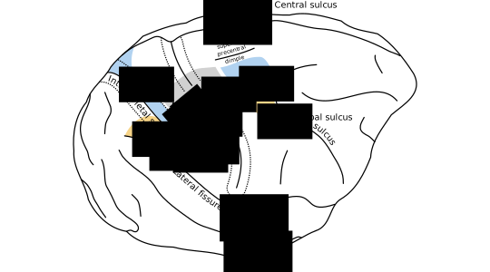
I'd also like to share two new illustrations from the introduction not published elsewhere:

Figure 1.1 

(high resolution PDF, SVG)


Figure 1.1: Anatomy of visually-guided reaching and grasping. During visually guided reaching and grasping, the arm and hand area of M1 coordinates with the dorsal and ventral premotor areas PMd and PMv. In this illustration, reciprocally connected motor and parietal areas are shaded in common colors. Premotor areas receive segregated streams of visual information from parietal cortex. Area PMd receives information about spatial geometry important for reaching from dorsal parietal areas (shaded in blue). Area PMv receives information about object geometry important for grasping from the parietal areas shaded in orange. Area M1 also receives feedback from somatosensory cortex (areas 3a,1,2, shaded in grey). Connections between parietal and premotor cortex are taken from Tanné-Gariépy et al. (2002), and anatomical boundaries of premotor areas are taken from Dum and Strick (2002).

Friday, March 20, 2015

Three unbiased estimators of spike-field coherence

[get notes as PDF]

In these notes we show a simplified expression for the Pairwise Phase Consistency (PPC) measure of Vinck et al. (2010). We illustrate it's relation to a bias-corrected spike-field coherence measure from Grasse et al. (2010), and discuss an third notion of spike-field coherence that is intermediate between the two. 

Here, we use the term "event-triggered" rather than "spike-triggered", because we want to apply these measures to neural events other than spikes (e.g. beta-frequency transients in motor cortex).

Pairwise Phase Consistency

Vinck et al. (2010) define Pairwise Phase Consistency (PPC) as the expected dot product between all pairs of (spike-triggered) phase measurements. 

\[\hat\Upsilon = \frac 2 {N(N-1)} \sum_{j=1..N-1} \sum_{k=j+1..N} \cos(\theta_j - \theta_k)\]

There is an alternative way to express PPC that is faster to calculate, and also reveals a relationship between PPC and similar alternatives. 

Wednesday, October 31, 2012

Sometimes the spike-triggered average is just as good as Poisson GLMs for spike-train analysis

(hopefully no major mistakes in this one; get PDF here)

The Poisson GLM for spiking data

Generalized Linear Models (GLMs) are similar to linear regression, but account for nonlinearities and non-uniform noise in the observations. In neuroscience, it is common to predict a sequence of spikes $Y=\{y_1,..,y_T\}$, $y_i\in\{0,1\}$, from a series of observations $X=\{\mathbf x_1,..,\mathbf x_T\}$, using a Poisson GLM:

$$ \begin{aligned} y_i &\sim \operatorname{Poisson}(\lambda_i\cdot\Delta t) \\ \lambda_i &= \exp\left( \mathbf a^\top \mathbf x_i + b \right) \end{aligned} $$

These models are fit by minimizing the negative log-likelihood of the observations, given the vector of regression weights $\mathbf a$ and mean offset parameter $b$:

Saturday, January 14, 2012

Bayesian approach to point-process generalized linear models

I've been learning about generalized linear models and Bayesian approaches for doing statistics on spike train data, in the Truccolo lab. Here are some notes on the subject. 

[get notes as a PDF]

In neuroscience, we are interested in the problem of how neurons encode, process, and communicate information. Neurons communicate over long distances using brief all-or-nothing events called spikes. We are often interested in how the spiking rate of a neuron depends on other variables, such as stimuli, motor output, or other ongoing signals in the brain. 

To model this, we consider spikes as events that occur at a point in time with an underlying variable rate, or conditional intensity, $\lambda$. There are many approaches to estimating $\lambda$. These notes cover point-process generalized linear models, and Bayesian approaches. These are closely related, and in some cases the same thing.

Tuesday, November 8, 2011

Point-Process Generalized Linear Models (PPGLMs) for spike train analysis

Get these notes as PDF here.

In neuroscience, we often want to understand how neuronal spiking relates to other variables. For this, tools like linear regression and correlation often work well enough. However, linear approaches presume that the underlying relationships are linear and the noise is Gaussian, neither of which are true for neural datasets. The Generalized Linear Model (GLM) extends linear methods to better account for nonlinearity and non-Gaussian noise.

GLMs for spike train analysis

We're interested in understanding how a neural spike train $y(t)$ relates to some other covariates $\mathbf x(t)$. In continuous time, a spike train is modeled as a train of impulses at each spike time $t_i$, $y(t)=\sum_i \delta(t-t_i)$. In practice, we always work in discrete time. It is common to choose a time step $\Delta t$ small enough so that at most one spike occurs in each time bin.

Two types of GLM that are common in spike train analysis:

  1. The Poisson GLM assumes that spikes arise from an inhomogeneous Poisson process with time-varying rate $\lambda(t)$ that depends log-linearly on the covariates $\mathbf x(t)$. In practice, it is common to treat the Poisson GLM in discrete time by assuming that the rate $\lambda(t)$ is constant within each time-bin:
\begin{equation*} \begin{aligned} y_t &\sim \operatorname{Poisson}(\lambda_t \cdot \Delta t) \\ \lambda_t &= \exp\left(\mathbf w^\top \mathbf x_t\right) \end{aligned} \end{equation*}
  1. The Bernoulli GLM models each time-bin of a binary, discrete-time spike train $y_t\in\{0,1\}$ as a Bernoulli "coin flip" with $\Pr(y{=}1)=p$.
\begin{equation*} \begin{aligned} y_t &\sim \operatorname{Bernoulli}(p_t) \\ p_t &= \frac 1 {1+\exp[-\mathbf w^\top \mathbf x(t)]} \end{aligned} \end{equation*}

Maximum likelihood

GLMs are typically estimated using maximum likelihood when testing how covariates $\mathbf x(t)$ influence spiking. (Other fitting procedures may be more appropriate when GLMs are used to model spiking dynamical systems.) The maximum likelihood procedure finds the weights $\mathbf w$ that maximize the likelihood of observing spike train $\mathbf y=\{y_1,..,y_T\}$, given covariates $\mathbf X = \{ \mathbf x_1,..,\mathbf x_T\}$, over all $T$ recorded time-bins.

\begin{equation*} \begin{aligned} \mathbf w = \underset{\mathbf w}{\operatorname{argmax}} \Pr( \mathbf y | \mathbf w, \mathbf X) \end{aligned} \end{equation*}

In practice, likelihood maximization is typically phrased in terms of minimizing the negative log-likelihood. Working with log-likelihood is more numerically stable, and the problem is phrased as minimization so that it is more straightforward to plug-in to off-the-shelf minimization code.

\begin{equation*} \begin{aligned} \mathbf w = \underset{\mathbf w}{\operatorname{argmin}} -\ln\Pr( \mathbf y | \mathbf w, \mathbf X) \end{aligned} \end{equation*}

Assuming observations are independent, the negative log-likelihood factors into a sum over time-points. Equivalently, one can minimize the average negative log-likelihood, over samples, $- \left< \ln\Pr( y_t | \mathbf w, \mathbf x_t) \right>$. The maximum likelihood parameters are typically solved for via gradient descent or the Newton-Raphson method . This requires computing the gradient and hessian of the negative log-likelihood.

Gradient and Hessian for the Poisson GLM

We can calculate the gradient and Hessian for the Poisson GLM by substituting the Poisson probability density function, $\Pr(y)=\lambda^y e^{-\lambda}/y!$, in to our expression for the negative log-likelihood:

\begin{equation*} \begin{aligned} -\left<\ln\Pr( y_t | \mathbf w, \mathbf x_t)\right> &= \left<\lambda_t - y_t \ln(\lambda_t) - \ln(y!)\right> \end{aligned} \end{equation*}

Because the term $\ln(y!)$ does not depend on $\mathbf w$, we can ignore it without affecting the location of our optimum. Substituting in $\lambda = \exp(\mathbf w^\top \mathbf x)$, we get:

\begin{equation*} \begin{aligned} \ell &= \left< \exp(\mathbf w^\top \mathbf x) - y_t \mathbf w^\top \mathbf x_t\right> \end{aligned} \end{equation*}

Finding weight $\mathbf w$ that minimize $\ell$ is equivalent to solving for the maximum-likelihood weights. The gradient and Hessian of of $\ell$ in $\mathbf w$ are:

\begin{equation*} \begin{aligned} \frac {\partial \ell} {\partial w_i} &= \left<[ \exp(\mathbf w^\top \mathbf x_t) - y_t] x_i \right> = \left<(\lambda_t - y_t) x_i \right> \\ \frac {\partial \ell} {\partial w_i \partial w_j} &= \left<[ \exp(\mathbf w^\top \mathbf x_t) ] x_i x_j \right> = \left< \lambda_t x_i x_j \right> \end{aligned} \end{equation*}

In matrix notation, these derivatives can then be written as:

\begin{equation*} \begin{aligned} \nabla \ell &= \langle \mathbf x( \lambda - y) \rangle \\ \mathbf H \ell &= \langle \lambda \mathbf x \mathbf x^\top \rangle \end{aligned} \end{equation*}

Gradient and Hessian for the Bernoulli GLM

The Bernoulli GLM is similar, with the observation probability given by the Bernoulli distribution $\Pr(y) = p^y (1-p)^{1-y}$

\begin{equation*} \begin{aligned} \left< -\ln\Pr( y_t | \mathbf w, \mathbf x_t) \right> &=- \left< y_t \ln(p_t) + (1-y_t) \ln(1-p_t) \right> \\&=- \left< y_t \ln\left(\tfrac{p_t}{1-p_t}\right) + \ln(1-p_t) \right> \end{aligned} \end{equation*}

Then, using $p = [1 + \exp(-\mathbf w^\top \mathbf x)]^{-1}$, i.e. $\mathbf w^\top \mathbf x = \ln[p/(1-p)]$, we get:

\begin{equation*} \begin{aligned} \ell &= \left< \ln[1+\exp(\mathbf w^\top \mathbf x_t)] - y_t \mathbf w^\top \mathbf x_t \right> \end{aligned} \end{equation*}

The gradient and Hessian of of $\ell$ in $\mathbf w$ are:

\begin{equation*} \begin{aligned} \frac {\partial \ell} {\partial w_i} &= \left< \left[\frac{\exp(\mathbf w^\top \mathbf x_t)}{1+\exp(\mathbf w^\top \mathbf x_t)} - y_t\right] x_i\right> \\&= \left<(p_t - y_t) x_i\right> \\ \frac {\partial \ell} {\partial w_i \partial w_j} &= \left<p_t (1-p_t) x_i x_j\right> \end{aligned} \end{equation*}

In matrix notation:

\begin{equation*} \begin{aligned} \nabla \ell &= \langle \mathbf x (p-y)\rangle \\ \mathbf H \ell &= \langle p(1-p) \cdot \mathbf x \mathbf x^\top \rangle \end{aligned} \end{equation*}

Iteratively reweighted least squares

PPGLMs can also be fit to spike train data using Iteratively Reweighted Least Squares (IRLS) . Recall that for a linear model $\mathbf y = \mathbf w^\top \mathbf x$, the Ordinary Least Squares (OLS) solution is:

$$ \mathbf w = \langle \mathbf x \mathbf x^\top \rangle^{-1} \langle \mathbf x \mathbf y^\top \rangle. $$

The IRLS approach phrases optimizing the parameters of the GLM in terms of repeated iterations of a reweighted least-squares problem. To derive this, first recall the definition of the Newton-Raphson update:

\begin{equation*} \begin{aligned} \mathbf w_{n+1} = \mathbf w_n - \mathbf H\ell(\mathbf w_n)^{-1} \nabla \ell(\mathbf w_n) \end{aligned} \end{equation*}

For the Poisson GLM, this is

\begin{equation*} \begin{aligned} \mathbf w_{n+1} = \mathbf w_n + \langle \lambda \mathbf x \mathbf x^\top \rangle^{-1}\langle \mathbf x (y-\lambda) \rangle \end{aligned} \end{equation*}

For e.g. the Poisson GLM, IRLS rewrites this as a least squares problem by defining weights $\lambda$ and pseudo-variables $z = \mathbf w^\top \mathbf x + \tfrac 1 \lambda (y - \lambda)$. We can confirm that the IRLS update is equivalent to the Newton-Raphson update:

\begin{equation*} \begin{aligned} \mathbf w_{n+1} &= \langle \lambda \mathbf x \mathbf x^\top \rangle^{-1} \langle \lambda \mathbf x z^\top \rangle \\&= \langle \lambda \mathbf x \mathbf x^\top \rangle^{-1} \left[ \langle \lambda \mathbf x [ \mathbf x^\top \mathbf w_n + \tfrac 1 \lambda (y-\lambda)] \rangle \right] \\&= \langle \lambda \mathbf x \mathbf x^\top \rangle^{-1} \left[ \langle \lambda \mathbf x \mathbf x^\top\rangle \mathbf w_n + \langle \mathbf x (y-\lambda) \rangle \right] \\&= \mathbf w_n + \langle \lambda \mathbf x \mathbf x^\top \rangle^{-1} \langle \mathbf x (y-\lambda) \rangle \end{aligned} \end{equation*}

Expected log-likelihoods

It's also possible to approximately fit $\mathbf w$ knowing only the mean and covariance of $\mathbf x$. This reduces computational complexity, since it avoids having to process the whole data matrix when optimizing $\mathbf w$. Previously, we calculated negative log-likelihood as an expectation over the data time-points. Here, we instead calculate these expectations based on a Gaussian model of the covariates $\mathbf x \sim \mathcal N(\mu_{\mathbf x}, \Sigma_{\mathbf x} )$. For example in the Poisson case, the gradient of the log-likelihood is :

\begin{equation*} \begin{aligned} \nabla \ell &= \langle \mathbf x( \lambda - y) \rangle = \langle \mathbf x \exp(\mathbf w^\top \mathbf x) \rangle - \langle \mathbf x y \rangle \end{aligned} \end{equation*}

The term $\langle\mathbf x y\rangle$ does not depend on $\mathbf w$, and can be computed in advance. The term $\langle \mathbf x \exp(\mathbf w^\top \mathbf x) \rangle$ has a closed-form solutions based on the log-normal distribution :

\begin{equation*} \begin{aligned} \langle \mathbf x \lambda \rangle &= [\langle \mathbf x \rangle + \mathbf w^\top \Sigma_{\mathbf x}] \langle\lambda\rangle \\ \langle \lambda \rangle &= \langle \exp(\mathbf w^\top \mathbf x) \rangle \\&= \exp( \mathbf w^\top \mu_{\mathbf x} + \tfrac 1 2 \mathbf w^\top \Sigma_{\mathbf x} \mathbf w) \end{aligned} \end{equation*}

The Hessian also has a closed form. This avoids having to recompute the re-weighted mean/covariances on every iteration. However, one still must calculate a mean and covariance initially. This approximation will only remain valid in the case that $\mathbf x$ is truly Gaussian. However, it can be used to pick an initial $\mathbf w_0$ before continuing with Newton-Raphson.

Edit: it seems like the Poisson GLM for Gaussian $\mathbf x$ might reduce to something like the spike-tiggered average in the limit where spikes are rare?