Thursday, June 22, 2017

Note: Marginal likelihood for Bayesian models with a Gaussian-approximated posterior

I first learned this solution from Botond Cseke . I'm not sure where it originates; It is essentially Laplace's method for approximating integrals using a Gaussian distribution, where the parameters of the Gaussian distribution might come from any number of various approximate inference approaches.

If I have a Bayesian statistical model with hyperparameters $\Theta$, with a no closed-form posterior, how can I optimize $\Theta$?

Saturday, February 4, 2017

System-size expansion and Gaussian moment closure for Quiescent-Active-Refractory model

Epilogue: These notes concern the system size expansion and moment closure later published as "Neural field models for latent state inference: Application to large-scale neuronal recordings" [pdf] (more) 

These notes derive the Kramers-Moyal system size expansion and approximate equation for the evolution of means and covariances of a single-compartment neural mass model with Quiescent (Q), Active (A), and Refractory (R) states. The derivations here are identical to the standard ones for the Susceptible (S), Infected (I), and Recovered (R) (SIR) model commonly used in epidemiology. 

[get these notes as PDF]

Thursday, January 26, 2017

Optogenetic stimulation shifts the excitability of cerebral cortex from type I to type II

Our new paper, Heitmann et al. [get PDF], is finally out! It's a collaboration between the theoretical neuroscientists Stewart Heitmann and Bard Ermentrout at the University of Pittsburgh, and the Truccolo lab at Brown University. 

This work could help us understand what happens when we stimulate cerebral cortex in primates using optogenetics. Modeling how the brain responds to stimulation is important for learning how to use this new technology to control neural activity.

Optogenetic stimulation elicits gamma (~50 Hz) oscillations, the amplitude of which grows with the intensity of light stimulation. However, traveling waves away from the stimulation site also emerge. It's difficult to reconcile oscillatory and traveling-wave dynamics in neural field models, but Heitmann et al. arrive at a surprising and testable prediction: 

The observed effects can be explained by paradoxical recruitment of inhibition at low levels of stimulation, which changes cortex from a wave-propagating medium to an oscillator. 

At higher stimulation levels, excitation overwhelms inhibition, giving rise to the observed gamma oscillations. 

Many thanks to Stewart Heitmann, Wilson Truccolo, and Bard Ermentrout. The paper can be cited as:

Heitmann, S., Rule, M., Truccolo, W. and Ermentrout, B., 2017. Optogenetic stimulation shifts the excitability of cerebral cortex from type I to type II: oscillation onset and wave propagation. PLoS computational biology, 13(1), p.e1005349.


Dissociation between sustained single-neuron spiking and transient β-LFP oscillations in primate motor cortex

Chapter two of my thesis has just been published! Rule et al. 2017 [PDF] explores the neurophysiology of beta (β) oscillations in primates, especially how single-neuron activity relates to population activity reflected in local field potentials (a.k.a. "brain waves").

Beta (~20 Hz) oscillations occur in frontal cortex. We've known about them for about a century, but still don't understand how they work or what they do. β-wave activity is related to "holding steady", so to speak. 

Beta oscillations are dysregulated in Parkinson's, in which movements are slowed or stopped. Beta oscillations are also reduced relative to slow-wave activity in ADHD, a disorder associated with motor restlessness and hyperactivity.

I looked at beta oscillations during movement preparation, where they seem to play a role in stabilizing a planned movement. I found that single neurons had very little relationship to the β-LFP brain waves. However! This appears to be for a good reason: the firing frequencies of neurons store information about the upcoming movement, and neurons firing at different frequencies cannot phase-lock together into a coherent population oscillation.

Anyone who's played in an orchestra knows that when notes are just slightly out of tune, you get interference patterns called beats. The same thing is happening in the brain, where many neurons firing at slightly different "pitches" cause β-LFP fluctuations, even though the underlying neural activity is constant.

This result provides a new explanation for how β-waves can appear as "transients" during motor steady-state: the fluctuations are cased by "beating", rather than changes in the β activity in the individual neurons. This differs from the prevailing theory for the origin of β transients in more posterior brain regions.

Many thanks to Carlos Vargas-Irwin, John Donoghue, and Wilson Truccolo. You can grab the PDF here. Please cite as

Rule, M.E., Vargas-Irwin, C.E., Donoghue, J.P. and Truccolo, W., 2017. Dissociation between sustained single-neuron spiking and transient β-LFP oscillations in primate motor cortex. Journal of neurophysiology, 117(4), pp.1524-1543.


Monday, June 6, 2016

Collective neural dynamics in primate motor cortex

As of the 29th of May, 2016, I officially have a Ph.D. in neuroscience! The thesis, Collective Neural Dynamics in Primate Motor Cortex, is available from the Brown University library [PDF].

I studied how single-neuron activity relates to large-scale collective neural dynamics during movement planning and execution. The thesis covers three research projects, which have been (will be) published as stand-alone papers:

  • Chapter 2, pp. 88-121: Contribution of LFP dynamics to spiking variability in motor cortex during movement execution. read more...
Rule, M.E., Vargas-Irwin, C., Donoghue, J.P. and Truccolo, W., 2015. Contribution of LFP dynamics to single-neuron spiking variability in motor c ortex during movement execution. Frontiers in systems neuroscience, 9, p.89.
  • Chapter 3, pp. 122:168: Dissociation between single-neuron spiking β-rhythmicity and transient β-LFP oscillations during movement preparation in primate motor cortex. read more…
Rule, M.E., Vargas-Irwin, C.E., Donoghue, J.P. and Truccolo, W., 2017. Dissociation between sustained single-neuron spiking and transient β-LFP oscillations in primate motor cortex. Journal of neurophysiology, 117(4), pp.1524-1543.
  • Chapter 4, pp. 169-213: Phase diversity and spatiotemporal wavedynamics in primate motor cortex local field potentials. read more…
Rule, M.E., Vargas-Irwin, C., Donoghue, J.P. and Truccolo, W., 2018. Phase reorganization leads to transient β-LFP spatial wave patterns in motor cortex during steady-state movement preparation. Journal of neurophysiology, 119(6), pp.2212-2228.

The introduction contains background on primate motor cortex (Chapter 1, pp. 7-88), including its constituent areas, how they connect with the rest of the brain, and how neurons connect to each-other within each area. It surveys what is known (as of 2016) about motor cortex population dynamics, LFP oscillations, and spatiotemporal waves. The section on statistical methods (Chapter 1.5, pp. 61-87) provides background for signal processing to extract single-neuron spikes and LFPs from multi-electrode array recordings. It also covers how to apply Generalized Linear Point-Process Models (PP-GLM) to analyze spiking neural data.

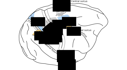
I'd also like to share two new illustrations from the introduction not published elsewhere:

Figure 1.1 

(high resolution PDF, SVG)


Figure 1.1: Anatomy of visually-guided reaching and grasping. During visually guided reaching and grasping, the arm and hand area of M1 coordinates with the dorsal and ventral premotor areas PMd and PMv. In this illustration, reciprocally connected motor and parietal areas are shaded in common colors. Premotor areas receive segregated streams of visual information from parietal cortex. Area PMd receives information about spatial geometry important for reaching from dorsal parietal areas (shaded in blue). Area PMv receives information about object geometry important for grasping from the parietal areas shaded in orange. Area M1 also receives feedback from somatosensory cortex (areas 3a,1,2, shaded in grey). Connections between parietal and premotor cortex are taken from Tanné-Gariépy et al. (2002), and anatomical boundaries of premotor areas are taken from Dum and Strick (2002).

Monday, May 9, 2016

More colors for Matplotlib

 
The default Matplotlib color scheme is not good. While searching for something better for my thesis, I stumbled upon Bridget Riley's painting "Gather" in the RISD museum. Is uses five colors: white, black, ochre, blue, turquoise, and a rust-colored red. But, from a distance they combine to create something far more vibrant. The blue and the turquoise hues are similar, so perhaps not the best to combine in a plot, but the others form an attractive and distinct pallet:

White #f1f0e9
Black #44525c
Rust #eb7a59
Ochre #eea300
Azure #5aa0df
Turquoise #00bac9

Surprisingly, when I ran this through a color-blindness simulator , some colors become even more distinct, so it is fairly color-blind friendly. I added colors to expand the pallet, to handle gradients and plots with extra lines.

Yellow #efcd2b
Moss #77ae64
Mauve #b56ab6
Magenta #cc79a7
Violet #8d5ccd
Indigo #606ec3
Viridian #11be8d
Chartreuse #b59f1a

These are less distinct, and not all combinations are color-blind friendly. Here's a bit of Python to define and tests these colors:

from pylab import *
from matplotlib import patches

WHITE = mpl.colors.to_rgb('#f1f0e9') RUST = mpl.colors.to_rgb('#eb7a59') OCHRE = mpl.colors.to_rgb('#eea300') AZURE = mpl.colors.to_rgb('#5aa0df') TURQUOISE = mpl.colors.to_rgb('#00bac9') BLACK = mpl.colors.to_rgb('#44525c') YELLOW = mpl.colors.to_rgb('#efcd2b') INDIGO = mpl.colors.to_rgb('#606ec3') VIOLET = mpl.colors.to_rgb('#8d5ccd') MAUVE = mpl.colors.to_rgb('#b56ab6') MAGENTA = mpl.colors.to_rgb('#cc79a7') CHARTREUSE = mpl.colors.to_rgb('#b59f1a') MOSS = mpl.colors.to_rgb('#77ae64') VIRIDIAN = mpl.colors.to_rgb('#11be8d')

GATHER = [WHITE,RUST,OCHRE,AZURE,TURQUOISE,BLACK] COLORS = [BLACK,WHITE,YELLOW,OCHRE,CHARTREUSE,MOSS,VIRIDIAN,TURQUOISE,AZURE,INDIGO,VIOLET,MAUVE,MAGENTA,RUST] CYCLE = [BLACK,RUST,AZURE,OCHRE,TURQUOISE,MAUVE,YELLOW,INDIGO] mpl.rcParams['axes.prop_cycle'] = mpl.cycler(color=CYCLE)

def test_panel(COLORS): ax = gca() NCOLORS = len(COLORS) axis('off') xlim(0,NCOLORS) ylim(NCOLORS,0) for j in range(NCOLORS): for i in range(NCOLORS): ax.add_patch(patches.Rectangle((i,j),1,1,linewidth=1, edgecolor='none',facecolor=COLORS[i])) ax.add_patch(patches.Rectangle((i+.25,j+.25),.5,.5,linewidth=1, edgecolor='none',facecolor=COLORS[j])) axis('equal')

figure(figsize=(6,3),dpi=200) subplots_adjust(0,0,1,1,0.1,0) subplot(111) test_panel(COLORS) savefig('colorblind_test_panel.png',bbox_inches='tight',pad_inches=0) </pre></div>

Two squences form decent color maps. They aren't perceptually uniform, but pass the color blindness simulator tests. Adding violet, mauve, and moss, to the original Gather pallet creates a hue wheel. This one flunks color-blindness test (see Crameri et al. ). Here they are in python:

riley2 = matplotlib.colors.LinearSegmentedColormap.from_list('riley2',
    [INDIGO,VIOLET,MAUVE,MAGENTA,RUST,OCHRE])

riley3 = matplotlib.colors.LinearSegmentedColormap.from_list('riley3', [OCHRE,CHARTREUSE,MOSS,VIRIDIAN,TURQUOISE,AZURE])

# Smoothed out mauve, violet, rust, ochre, moss, turquoise, azure, in a loop hues = ['#8c62cc', '#9560c8', '#9e62c3', '#a765be', '#b068b6', '#bb6caa', '#c66f98', '#d27384', '#dd7670', '#e67c5c', '#ea8348', '#ec8b34', '#ec9421', '#e99c13', '#dea212', '#c9a620', '#b0a934', '#96ab4a', '#7cae60', '#62b076', '#48b38c', '#2eb5a2', '#1ab7b6', '#12b6c5', '#1cb2ce', '#2dadd4', '#41a7d8', '#529fdb', '#6194db', '#6d86d8', '#7977d4', '#836ad0'] riley = matplotlib.colors.LinearSegmentedColormap.from_list('riley',hues)

# Make new maps behave like native Matplotlib maps plt.register_cmap(name='riley2',cmap=riley2) plt.register_cmap(name='riley3',cmap=riley3) plt.register_cmap(name='riley' ,cmap=riley )

# Show as figure figure(figsize=(5,1),dpi=300) subplot(311) imshow([linspace(0,1,256)],cmap='riley2',aspect='auto') axis('off'); tight_layout() subplot(312) imshow([linspace(0,1,256)],cmap='riley3',aspect='auto') axis('off'); tight_layout() subplot(313) imshow([linspace(0,1,256)],cmap='riley',aspect='auto') axis('off'); tight_layout() subplots_adjust(hspace=0.3) savefig('moremaps.png') </pre></div>