Consider a stochastic, binray, linear-nonlinear unit, with spiking output $s$, synaptic inputs $\mathbf x$, weights $\mathbf w$, and bias (threshold) $b$:
\begin{equation}\begin{aligned} s &\sim\operatorname{Bernoulli}[p = \Phi(a)] \\ a &= \mathbf w^\top \mathbf x + b, \end{aligned}\end{equation}where $\Phi(\cdot)$ is the cumulative distribution function of a standard normal distribution. Note that $\Phi(\cdot)$ can be rescaled to closely approximate the logistic sigmoid if desired. Assuming the mean $\mu$ and covariance $\Sigma$ of $\mathbf x$ are known, can we obtain the mean and covariance of $s$?
The wrong way: A small-variance approximation
It is common to model the stochastic response in terms of the mean-field (deterministic) transfer function $\Phi(a)$, plus a small correction assuming that the variance in $a$ is small. This works acceptable for weakly-nonlinear units, like Poisson, but fails for Bernoulli units.
One can approximate the variance of the spiking $s$ output as the sum of the variance from the Bernoulli sampling, and the variance in the Bernoulli rate itself. The variance of a Bernoulli variable is $p(1-p)$, and the variance in $p$ itself can be obtained from a locally-linear Gaussian approximation as the variance of the activation, multiplied by the slope of the effective transfer function $f'(\mu_a)$:
\begin{equation} \begin{aligned} \sigma^2_s & = p (1-p) + f'(\mu_a)^2 \cdot \sigma_a^2 \end{aligned} \end{equation}This approximation is convenient, and works for generic nonlinearities (not just $\Phi(a)$). More generally, we can use the linear-Gaussian approximation to estimate the covariance ($\Sigma_s$) of a population of output neurons driven by shared (noisy) inputs:
\begin{equation} \begin{aligned} \mu_s &= f(W\mu_x + B) \\ \Sigma_s &= J \Sigma_x J^\top + Q \\ J &= \partial_x \mu(\left<x\right>) \\ Q &= \operatorname{Diag}\left[\mu(x) \left(1-\mu(x)\right)\right], \end{aligned} \end{equation}Where $W$ denotes a matrix of input weights, $B$ denotes a vector of per-unit biases, and $\vec\mu(x)$ reflects a (mean-field estimate) of the vector of output mean-rates.
This approximation arises from a locally-linear approximation of the nonlinear transfer function $f$, which transforms correlated inputs $\Sigma_x$ according to the jacobian $J$ of the firing-rate nonlinearity. This also includes a Gaussian (diffusive) approximation of the noise arising from Bernoulli sampling, $Q$, which is equal to $p(1-p)$. A similar result holds for the Poisson (low firing-rate limit), for which $Q=\operatorname{Diag}[\vec\mu(x)] \Delta t$.
Additional corrections can be added, for example accounting for the effect of variance on $\vec\mu(x)$ for estimating the noise source term $Q$, or providing additional corrections based on higher-order moments or moment-closure approximations thereof.
Similar locally-quadratic approximations for noise have been advanced in the context of chemical reaction networks (Ale et al. 2013). Rule and Sanguinetti (2018) and Rule et al (2019) use this approach in spiking neuron models, and Keeley et al. (2019) explored spiritually similar quadratic approximations for point-processes.
The small-variance correction is essentially the first term in a family of series expansions, which use the Taylor expansion of the firing-rate nonlinearity to capture how noise is transformed from inputs to outputs. In the case of linear-nonlinear-Bernoulli neurons, approximations based on series expansions like this have poor convergence. Polynomial approximations to $\Phi$ diverge as the activation becomes very large or very small, whereas the sigmoidal nonlinearity is bounded. Global approximations are therefore desirable when the variance of the input is large.
A better way: Dichotomized Gaussian (probit) moment approximation
Global approximations have been presented elsewhere for other types of firing nonlinearity. Echeveste et al. (2019) used exact solutions for propagation of moments for rectified-polynomial nonlinearities (Hennequin and Lengyel 2016). Rule and Sanguinetti (2018) also illustrate an example with exponential nonlinearities.
These approaches fall under the umbrella of "moment-based methods", and entail solving for the propagation of means and correlations under some distributional anstaz (often Gaussian, although see Byrne et al. 2019 for an important application using circular distributions). In general, there are few guarantees of accuracy for these methods (Schnoerr et al. 2014, 2015, 2017), although they are often empirically useful.
Moment approximations fair poorly for the linear-nonlinear-Bernoulli neuron. However, when one takes the firing-rate nonlinearity to be the CDF of the standard normal distribution, global approximations are possible. This yields suitable approximations for other sigmoidal nonlinearities, provided that these nonlinearities can be approximated by the normal CDF under a suitable change of variables.
The variance and covariances in a population of dichotomized Gaussian neurons can be expressed in terms of the multivariate normal CDF. To derive the population covariance, consider a single entry which reflects the covariance between a pair units.
\begin{equation} \begin{aligned} \Sigma_{12} &= \left<(s_1-p_1)(s_1-p_2)\right> \\ &= \left<s_1 s_2\right> - p_1 p_2 \\ \left<s_1 s_2\right> &= \Pr(s_1 = s_2 = 1) \end{aligned} \end{equation}If $a=w^\top x+b$ is the activation, and $u=a+\xi$ is the activity combined with zero-mean unit-variance threshold noise $\xi$, we can evaluate $\left<s_1 s_2\right>$ by considering the joint distribution of $u_1$ and $u_2$ as Gaussian (for a numerical recipe see Drezner and Wesolowsky 1989; numerical implementations are provided in standard computing packages, e.g. Matlab or Scipy in Python):
\begin{equation} \begin{aligned} \left<s_1 s_2\right> &= \Pr(u_1>0\text{ and }u_2>0). \\ u&\sim\mathcal N(\mu_u,\Sigma_u) \\ \mu_u &= \mu_a \\ \Sigma_u &= \Sigma_a + \operatorname{I}. \end{aligned} \end{equation}A numerical solution in terms of the bivariate Gaussian CDF is useful for propagating activity, but challenging for building a differentiable model suitable for optimization. However, practical approximations exist.
Faster approximations to dichotomized Gaussian moment approximation
For a single neuron, the mean and variance of the spiking output are those of a $\operatorname{Bernoulli}(p)$ distribution, with probability $p=\Pr(s=1)$. The mean rate $\mu_s$ is equal to the probability of firing ($p$), and the variance $\sigma^2_s$ is equal to $p(1-p)$ (Fig a).
Binary spiking units with a Gaussian CDF nonlinearity $\Phi(\cdot)$ can be modeled as a thresholded Gaussian noise source. When this noise is above a certain threshold ($-a$), the unit emits a "1", otherwise, a "0". This makes it easy to model the effect of additional noise (variance) in the synatpic activation "a". This extra noise simply sums with the existing Gaussian noise in the model of the stochastic spiking.
The spiking probability $p$ of a dichotomized-Gaussian unit being driven by noisy, Gaussian inputs can be obtained by treating the effect of noise in activation ($\sigma^2_a$) as a decrease in gain:
\begin{equation} \begin{aligned} a &\sim \mathcal N(\mu_a,\sigma^2_a) \\ p &= \left<\Phi(a)\right>= \Phi\left(\gamma \mu_a\right) \\ \gamma &= \frac{1}{\sqrt{1+\sigma^2_a}} \\ \mu_s &= p \\ \sigma^2_s &= p(1-p) \end{aligned} \end{equation}To see this in more depth, observe that the variance in the spiking output $\sigma^2_s$ is a combination of the average spiking variance $\sigma^2_{\text{noise}}=\left<p(1-p)\right>$, plus whatever input noise in the firing rate ($\sigma_p^2$) is passed through the nonlinearity. In the dichotomized Gaussian model of a linear-nonlinear-Bernoulli neuron, we find that $\sigma^2_s \approx \mu_p(1-\mu_p)$:
\begin{equation} \begin{aligned} \sigma^2_{\text{noise}} &= \left< p(1-p) \right> \\&=\left<p\right> - \left<p^2\right> \\&=\mu_p-(\mu_p^2+\sigma_p^2) \\&=\mu_p(1-\mu_p)- \sigma_p^2 \\ \\ \sigma_p &\approx \sigma_a \cdot \left< \partial_a \Phi(a) \right> \\&= \sigma_a \cdot \partial_a \left< \Phi(a) \right> \\&= \sigma_a \cdot \partial_a \Phi(\mu_a\gamma) \\&= \sigma_a \cdot \phi(\mu_a\gamma) \cdot \gamma \\ \\ \sigma^2_s &= \sigma^2_p + \sigma^2_{\text{noise}} \\ &= \sigma^2_p + [\mu_p(1-\mu_p) - \sigma_p^2] \\& = \mu_p(1-\mu_p). \end{aligned} \end{equation}This generalizes to the multivariate case, and provides an approximation for how correlations in inputs propagate to correlations in the output:
\begin{equation} \begin{aligned} \Sigma_s &= \Sigma_p + \Sigma_{\operatorname{noise}} \\ \Sigma_p &\approx J \Sigma_a J^\top \\ \Sigma_{\operatorname{noise}} &\approx \operatorname{Diag}[p(1-p) - \sigma^2_p] \\ J &= \operatorname{Diag}\left[\phi(\gamma\mu_a)\cdot\gamma\right] \\ p &= \Phi(\gamma\mu_a), \\ \gamma &= \left(1+\operatorname{Diag}[\Sigma_a]\right)^{-\frac 1 2} \end{aligned} \end{equation}The accompanying figure shows a toy example of variance approximation, using a network of three neurons (Fig. b). Compared to the small-variance approximation, the approximation derived for the dichotomized Gaussian case provides a better approximation of the moments of the output, and accounts for how noise in the input propagates to the output (Fig. c).
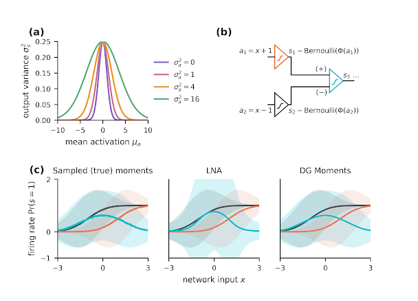
Figure: variance propagation in the dichotomized Gaussian neuron (a) For a single neuron, the effect of input variability ($\sigma^2_a$) can be viewed as a modulation of the gain of the nonlinear transfer function. The output variance is then similar to that of a Bernoulli distribution. (b) In a feed-forward network of nonlinear stochastic neurons, noise propagates to downstream neurons, affecting the computational properties of the circuit. (c) The output (blue) of this circuit is stochastic, and noise in the first layer (black, red) propagates to the output (left panel: Monte-Carlo samples, shaded = 5-95${}^{th}$ percentile), but can be modeling in a differentiable way using moment approximation. The small variance approximation (linear noise approximation or LNA, in this case: middle ) loses some accuracy for small circuits, since the is very little averaging to attenuate spiking noise. The moment approximation using a dichotomized Gaussian (DG) model is more accurate (right).
No comments:
Post a Comment